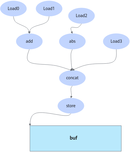
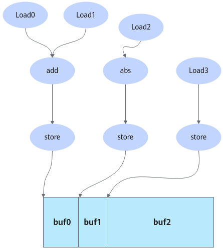
Schedule

Loop Fusion

Loop fusion is an important loop transformation technique. It reconstructs the loop structure to reduce memory access times, reduce the control overhead, improve data locality, and pave the way for subsequent optimization. In this way, the program execution efficiency is improved without changing the computation result.

For example, assume that there are two layers of loops:

1
2
3

for i in range(N):
    for j in range(M):
        C[i][j] = A[i][j] + B[i][j]

Add is a pure elewise operation. Therefore, it can be fused into a linear loop.

1
2
3
4

for fused in range(N * M):
    i = fused // M
    j = fused % M
    C[i][j] = A[i][j] + B[i][j]

The corresponding AscIR expression is as follows:

 1
 2
 3
 4
 5
 6
 7
 8
 9
10
11
12
13
14
15
16
17
18
19
20
21
22
23

z0 = graph.create_axis("z0", N)
z1 = graph.create_axis("z1", M)
Load load0("load_0");
load0.x = data0.y;
load0.attr.sched.axis = {z0.id, z1.id};
load0.y.axis = {z0.id, z1.id};
load0.y.repeats = {N, M};
load0.y.strides = {M, 1};

Load load1("load_1");
load1.x = data1.y;
load1.attr.sched.axis = {z0.id, z1.id};
load1.y.axis = {z0.id, z1.id};
load1.y.repeats = {N, M};
load1.y.strides = {M, 1};

Add add("add");
add.x1 = load0.y;
add.x2 = load1.y;
add.attr.sched.axis = {z0.id, z1.id};
add.y.axis = {z0.id, z1.id};
add.y.repeats = {N, M};
add.y.strides = {M, 1};

After loop fusion:

 1
 2
 3
 4
 5
 6
 7
 8
 9
10
11
12
13
14
15
16
17
18
19
20
21

Load load0("load_0");
load0.x = data0.y;
load0.attr.sched.axis = {z0z1.id};
load0.y.axis = {z0z1.id};
load0.y.repeats = {N * M};
load0.y.strides = {1};

Load load1("load_1");
load1.x = data1.y;
load1.attr.sched.axis = {z0z1.id};
load1.y.axis = {z0z1.id};
load1.y.repeats = {N * M};
load1.y.strides = {1};

Add add("add");
add.x1 = load0.y;
add.x2 = load1.y;
add.attr.sched.axis = {z0z1.id};
add.y.axis = {z0z1.id};
add.y.repeats = {N * M};
add.y.strides = {1};

TilingCase Generation

In automatic fusion, tiling solution space generation is the key to efficient compute scheduling. Its core objective is to provide diversified tiling strategy options for complex compute tasks, so that the optimizer can select the optimal solution. Simply speaking, the tiling solution space generation process can be considered as a systematic enumeration of the tiling possibility of input data or compute tasks. Each solution space is called a TilingCase.

The tiling mode design is closely related to the operator implementation features. To systematically enumerate the tiling strategies for diversified operators, the operators are abstracted into nine compute types (compute and view operators in the following figure) based on the operator implementation features. Operators of the same compute type have similar compute logic and data access modes. In this way, they can share the same tiling strategy framework.

Figure 1 Tiling strategies

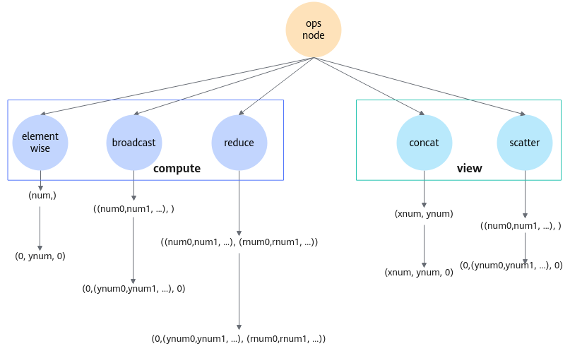
To materialize the policy framework, the axes of an operator are normalized and grouped. All axes are grouped into three dimension groups (xgroup, ygroup, and rgroup). They are defined as follows:

• xgroup: group designed for view operators such as Concat. Here, the Concat is used as an example. The axes before the Concat axis are grouped into xgroup, and the Concat axis and its subsequent axes are grouped into ygroup.
• ygroup: a loop axis group for the Elementwise and Broadcast operators.
• rgroup: Reductions usually have special tiling requirements on the reduced axis. Therefore, all reduced axes are placed in rgroup.

The core reason for introducing xgroup, ygroup, and rgroup is to support the dual tiling requirements in complex scenarios. For example, in a computational graph that contains reduce fusion, ygroup controls the loop tiling in the elementwise direction, and the axis in rgroup controls the loop tiling in the reduce direction.

After the axis grouping of a single operator is complete, the grouping policies of all operators in the computational graph need to be merged based on the preset merge rule (Merge). The merging result is used as a unified tiling strategy applicable to all operators in the graph, providing a basis for subsequent solution space generation.

The preceding grouping and merging mechanism can be used to:

• Filter out the tiling modes applicable to all nodes in the computational graph to form an effective TilingCase.
• Check whether the tiling groups of different AscGraphs can be successfully merged to verify the fusion of the two graphs.

The following case is used as an example to describe the principle of generating a TilingCase through tiling grouping and merging:

 1
 2
 3
 4
 5
 6
 7
 8
 9
10
11
12
13
14
15
16
17
18
19
20
21
22
23
24
25

z0 = graph.create_axis("z0", s0)
z1 = graph.create_axis("z1", s1)
data = ascir.ops.Data('data', graph)
data.y.dtype = ascir.dtypes.float32
# Declare the load operator.
load = ascir.ops.Load('load')
load.attr.sched.axis = [z0, z1] # Scheduling axis
load.x = data.y
load.y.axis = [z0, z1] # Output axis of the tensor
load.y.size = [s0, s1] # Tensor output size
load.y.strides = [s1, 1] # Output stride of the tensor
# Declare the abs operator.
abs = ascir.ops.Abs('abs')
abs.attr.sched.axis = [z0, z1]
abs.x = load.y
abs.y.axis = [z0, z1]
abs.y.size = [s0, s1]
abs.y.strides = [s1, 1]
# Declare the max operator.
max = ascir.ops.Max('max')
max.attr.sched.axis = [z0, z1]
max.x = abs.y
max.y.axis = [z0, z1]
max.y.size = [s0, 1] # Perform the reduction on the z1 axis.
max.y.strides = [1, 0]

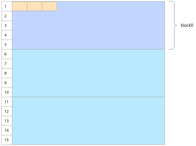
abs is an elewise operator. The computation of each axis is the same. Therefore, as long as the memory is continuous, multiple axes can be merged into one axis for tiling. As shown in Figure 2, block partitioning is performed on the axis, 15 is tiled into three blocks, and block 0 is marked in purple. Then, tiling is performed in block 0. In this case, the tiling block does not fully occupy the part allocated to block 0. Therefore, a for loop needs to be added to the block.

Figure 2 Tiling of elewise operators

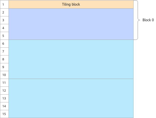
The tiling of the reduce class is complex, and dual tiling is required. The elewise axis is in the row direction, and the reduced axis is in the column direction. First, blocks are divided in the row direction, a loop is written in the block, and then a for loop is added in the column direction.

Figure 3 Tiling of reduce operators

Rule combination for TilingGroup:

1

()(z0,z1)() Merge ()(z0)(z1) => ()(z0)(z1)

The abs operator's (z0, z1) axes that originally belong to the ygroup are tiled. The z1 axis is moved to the rgroup. The core purpose of this adjustment is to ensure that the abs operator and subsequent reduce operators use the same tiling strategy.

Parallel Optimization

• Loop Splitting

  The core role of loop splitting is to introduce new loop levels, thereby clearly identifying outer loops suitable for parallelism and inner loops suitable for vectorization.

  For each tiling case, the axes in xgroup, ygroup, and rgroup are split into ub_out and ub_in.

  

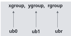
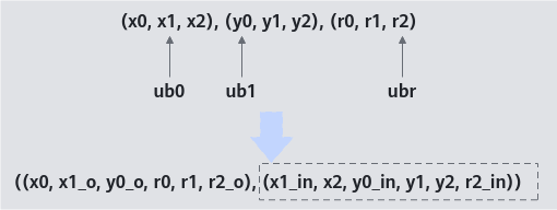
  For example, for {z0, z1, z2}, z1 is split into z1T and z1t. z1T is ub_out, and z1t is ub_in.

• Vectorization

  Vectorization is a key technology that uses the hardware single-instruction multiple-data (SIMD) stream processing unit to improve the data parallel computation efficiency. It converts single-element operations into vector operations, significantly reducing the number of instruction executions and improving hardware utilization.

  For example, for the following loop:

  1 2 3

  for (int i = 0; i < 256; i++) { c[i] = a[i] + b[i]; }

  Non-vectorized execution needs 256 addition instructions, but vectorized execution needs just one.

  After an axis is selected as the ub splitting axis in each group, ub_in and its inner axis serve as the vectorization axis. Since the groups are generated in the order of x, y, and r, the vectorization axis generated this way may have a different axis order from the memory layout, which can lead to non-contiguous movement. Therefore, the axis order needs to be rearranged based on the output axis order.

  

  For example, if the axis order of the output tensor is (a, b, c, d) and the axis groups are (a, c) and (b, d)(), the vectorization axis groups generated in this order are (a_in, c, b_in, d), which need to be adjusted to (a_in, b_in, c, d).

  

  In the Schedule phase, the same vectorization axis is set for the entire graph. For some APIs, not all vectorization axes can be vectorized due to instruction restrictions. In this case, in the CodeGen phase, you need to perform the for loop operation on the axes that cannot be vectorized.

  For example, if the vectorization axis is [z1, z2, z3], it has three layers of loops. If the instruction supports three layers of loops, the vectorization axis can be specified as vector[z1, z2, z3]. However, if the instruction supports only two layers of loops, CodeGen needs to provide the following code:

  1 2 3

  for (i in z1) { vector[z2,z3] }

• Loop fusion and loop binding

  Loop fusion and loop binding are often used together for optimization. In the loop splitting phase, the ub_out axis is generated in each group.

  1. Fuse all non-reduced axes into one, and fuse all reduced axes into one to reduce the number of nested loops.
  2. Split the fused loop to obtain outer and inner layers.
  3. Bind the split outer loop to multiple blocks to implement parallelism, with the inner layer sequentially handling the assigned workload.

  

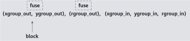
  For example, for {z0, z1T, z1t, z2}, z0 and z1T are fused into a single axis (z0z1T), which is then split across cores. Since the fused axis size can exceed the number of available AI Cores, a single round of core mapping is insufficient. Therefore, after core allocation, z0z1T undergoes an additional layer of loop, dividing it into z0z1TB and z0z1Tb. The exact values of these divisions are calculated by Auto Tiling during the tiling phase.

Memory Optimization

Currently, memory resources are reused based on node reference relationships. To improve the reuse effect, memory of similar sizes is allocated to a group and then reused within the group.

The pseudocode for memory reuse is as follows:

 1
 2
 3
 4
 5
 6
 7
 8
 9
10
11
12
13

for (node in all nodes) {
  for (output in node.outputs) {
    // Mark the number of tensor dependencies.
    output->sch.depends = output->anchor->GetPeerInDataNodesSize();
    // try reuse from free queue
  }
  for (input in node.inputs) {
    input->sch.depends--;
    if (input->sch.depends == 0) {
        Enque(input->opt.reuse_id); // Mark the tensor as a freeTensor, which can be reused by subsequent nodes.
    } 
  }
}

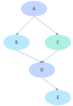
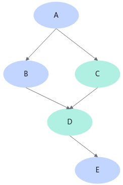
For some APIs, the output can directly reuse the input. For these APIs, in-place reuse can be adopted, that is, the output directly reuses the input memory. As shown in the following figure, three memory blocks are required before in-place reuse.

Figure 4 Before memory reuse

After in-place reuse, only two memory blocks are required.

Figure 5 After memory reuse

Multi-template Generation

A computational graph may be implemented in multiple ways. Take the tail-axis concat as an example. You can perform the ub_concat operation on multiple small packets in the Unified Buffer to form a large packet and then move the large packet out. Alternatively, you can directly convert the packets into discontinuous packets and move and reorder them in the global memory. The former can significantly improve the memory movement efficiency of the Memory Transfer Engine (MTE) for the AI Core in small-shape scenarios, thereby achieving better performance. However, the ub_concat operation requires full loading of the inner axis. As a result, this operation does not apply to certain scenarios. If the template to be selected cannot be determined in the schedule phase, a general template applicable to any shape and a performance optimization template for specific scenarios are generated. The Auto Tiling module determines the template to be used in the tiling phase.

• Unified Buffer concat template:

  

• Graph modification template: