Fusion Policy Solving

After the operations in Fusion Condition Check are completed, if two nodes can be fused, multiple fusion results (for example, fusion policy 1 and fusion policy 2 in the following figure) may be generated. When there are multiple fusion policies, you need to determine the optimal policy to be used.

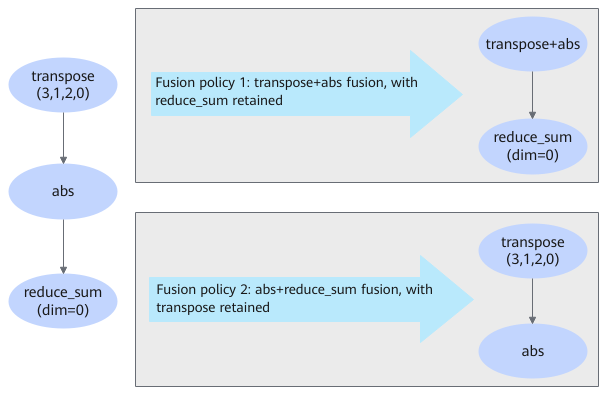
It is difficult to compute the optimal fusion policy of the entire graph. The main reasons are as follows:

1. The algorithm complexity may be high. One feasible approach is to use dynamic programming, though achieving a complexity of nlog(n) remains challenging.
2. The performance estimation model is inaccurate. Before the actual test on the board, it is difficult to accurately determine the actual post-fusion performance.

Due to the preceding reasons, pursuing a strict global optimal solution inevitably involves a large number of entire graph fusion attempts and board tests, resulting in a significant increase in time complexity. Therefore, the score and greedy simple fusion policy solving algorithm are used currently. Specifically, pair the nodes that can be fused on the graph, and determine whether the nodes can be fused one after another. If the nodes can be fused, sort the nodes based on the score (to determine the fusion sequence), and then fuse the nodes in sequence. After the first round of fusion, repeated operations are performed to attempt multi-round fusion of the nodes. A maximum of 10 rounds of fusion are supported. The fusion scoring rules are as follows:

1. Compute the saved memory size (use symbols to compare the size. The larger the size, the higher the priority).
2. Compute the proximity between nodes (use the difference of topological sequence IDs. The smaller the difference, the higher the priority).

Sorting priority:

Compare the memory sizes first. If the memory sizes are the same, compare the proximity. If the proximity is also the same, sort the nodes in ascending order of the topological sequence and perform deduplication to obtain the node pairs that can be fused. The nodes are then fused in this sequence.

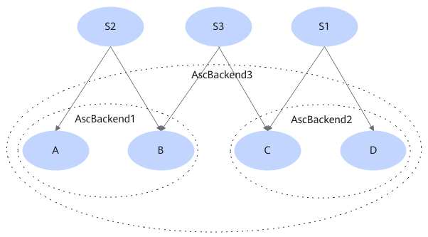
Figure 2 and Figure 3 are used as examples to describe how to use the greedy algorithm.

In Figure 2, A, B, C, and D form the AB, BC, and CD fusion node pairs. After sorting, the fusion sequence is determined. Assume that the fusion sequence is CD first and AB second. After the fusion, the paris become CD and AB. When BC is fused, B has become AB and C has become CD. Finally, AB+CD fusion is performed.

In Figure 3, if the sorting sequence is AB first and BC second, the fusion process changes. AB is fused first. In BC fusion, B has become AB, and AB+C is fused. Similarly, CD is fused into ABC+D.

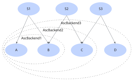
The final fusion results in both scenarios are the same, that is, ABCD. However, if A and D cannot be fused, the actual results will be different. The results in Figure 2 are AB and CD, and the results in Figure 3 are ABC and D. This indicates that the fusion sequence change leads to different fusion processes and results. The current algorithm also has limitations. The current greedy algorithm considers only local optimality, which may not be optimal globally. For example, if A and D cannot be fused, CD is fused first, ABC may not be fused. From the global perspective, this may not be the optimal policy.