Multi-Instance Deployment

Function Description

Deploying multiple instances accelerates computing when a node needs significant computing resources.

Constraints

After multiple instances are deployed, the computing timing between instances is inconsistent. You may need to enable data alignment to ensure data pairing.

How to Use

For instructions on enabling multiple instances, see Specifying the Deployment Location of the DataFlow Node.

Two applicable implementation modes are provided for different scenarios, as shown in the following table.

• Parallel mode 1: multi-instance parallelism between requests
  Figure 1 Multi-instance parallelism between requests
  

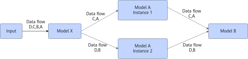
  The DataFlow model is a serial pipeline consisting of Model X, Model A, and Model B. Since Model A involves heavy computation, two instances are deployed for Model A to accelerate processing. After data flows A, B, C, and D pass through Model X, they are distributed to the two instances of Model A in round-robin mode based on transaction ID: data A and C are routed to instance 1, while data B and D are routed to instance 2. Model B then aggregates all processed data.

• Parallel mode 2: request splitting for multi-instance acceleration
  This scenario requires additional logic for data splitting and data merging. You can specify BalanceConfig during output to implement balanced data distribution and control output distribution and aggregation. (This capability does not support the py_flow annotation execution mode currently.)

  Figure 2 Request splitting for multi-instance acceleration
  

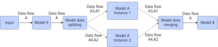
The original DataFlow model consists of Model X, Model A, and Model B connected sequentially. Model A is the latency bottleneck due to its heavy computation. To reduce end-to-end latency, Model A is replicated into multiple instances for parallel acceleration. The detailed procedure is as follows:

1. Request data A enters the model data splitting module through Model X and is split into four pieces of data (A1, A2, A3, and A4). Perform this operation according to your service logic. Include relevant data identifiers such as DataId or DataName in the split data for easy tracking and future processing.
2. A1 and A3 are sent to instance 1 of Model A, and A2 and A4 are sent to instance 2 of Model A.
3. The processed A1, A2, A3, and A4 are sent to the model data merging module and merged into data A.
4. Data A is sent to Model B.

The following is an example of data distribution.

The following describes the data distribution logic for the split data A1, A2, A3, and A4.

 1
 2
 3
 4
 5
 6
 7
 8
 9
10
11
12
13
14
15
16
17
18
19
20
21
22

# Graph construction phase
flow_node.set_balance_scatter()

# UDF output mode 1: batch output, which is applicable to the scenario where data is split only once.
cfg = ff.BalanceConfig(1, 4, ff.AffinityPolicy.NO_AFFINITY) # The meanings are as follows: row_num=1, col_num=4 (four pieces of data in total), affinity_policy=ff.AffinityPolicy.NO_AFFINITY (non-affinity)

cfg.set_data_pos([(0, 0), (0, 1), (0, 2), (0, 3)]) # The pos values corresponding to A1, A2, A3, and A4 are {0, 0}, {0, 1}, {0, 2}, and {0, 3}, respectively.
context.set_multi_outputs(0, [msg0, msg1, msg2, msg3], cfg)
# UDF output mode 2: single output. This mode is applicable to scenarios where users split data into individual pieces, enabling earlier split data to be processed in advance.
cfg = ff.BalanceConfig(1, 4, ff.AffinityPolicy.NO_AFFINITY)
# Distribute the split msg0.
cfg.set_data_pos([(0, 0)])
context.set_output(0, msg0, cfg)
# Distribute the split msg1.
cfg.set_data_pos([(0, 1)])
context.set_output(0, msg1, cfg)
# Distribute the split msg2.
cfg.set_data_pos([(0, 2)])
context.set_output(0, msg2, cfg)
# Distribute the split msg3.
cfg.set_data_pos([(0, 3)])
context.set_output(0, msg3, cfg)

The following is an example of data merging:

1
2
3
4
5
6
7

# Graph construction phase
flow_node.set_balance_gather()
# Set BalanceConfig of the UDF.
cfg = ff.BalanceConfig(1, 4, ff.AffinityPolicy.ROW_AFFINITY)# The meanings are as follows: row_num=1, col_num=4 (four pieces of data in total), and affinity_policy=ff.AffinityPolicy.ROW_AFFINITY (affinity by row).
# Each instance distributes the data of the same row to the same subsequent target node. (If the data merging node is a single node, you do not need to specify BalanceConfig.) The data merging module merges the received data.
cfg.set_data_pos([(0, 0)])
context.set_output(0, msg0, cfg)