Getting Started with Performance Analysis in Offline Inference Scenarios

Collecting, Parsing, and Exporting Profile Data ( Ascend EP )

1. Log in to the operating environment and run the following command to collect, parse, and export profile data in one click:

   msprof --output=<path> <app>

   Example command:

   msprof --output=/home/projects/output /home/projects/MyApp/out/main

   Table 1 Command-line options

   Option	Description	Optional/Required
   --output=<path>	Directory for storing the collected profile data. The value defaults to the current directory.	Optional
   <app>	Add the AI task execution command to the end of the msprof command as required to pass the user application or execution script.	Required

   After the command is executed, find the PROF_XXX directory generated in the directory specified by --output. This directory stores the automatically parsed profile data. (The following shows only the profile data.)

   1 2 3 4 5 6 7 8 9 10 11 12 13 14

   ├── host // Save the original data. You can ignore this step. ... │ └── data ├── device_{id} // Save the original data. You can ignore this step. ... │ └── data ... ├── msprof_*.db ├── mindstudio_profiler_output ├── msprof_{timestamp}.json ├── step_trace_{timestamp}.json ├── xx_*.csv ... └── README.txt

2. Access the mindstudio_profiler_output directory to view corresponding profile data files.

   For details about the files collected by default, see Table 2.

   Table 2 Profile data files collected by msprof by default

   File Name	Description
   msprof_*.db	.db file that aggregates all profile data. You are advised to use MindStudio Insight to analyze the .db file. For details, see MindStudio Insight User Guide.
   msprof_*.json	Timeline report.
   step_trace_*.json	Iteration trace data, which records the time required for each iteration. This profile data file does not exist in single-operator scenarios.
   op_summary_*.csv	AI Core and AI CPU operator data.
   op_statistic_*.csv	Number of times that the AI Core and AI CPU operators are called and the time consumption.
   step_trace_*.csv	Iteration trace data. This profile data file does not exist in single-operator scenarios.
   task_time_*.csv	Task Scheduler data.
   fusion_op_*.csv	Operator fusion summary in a model. This profile data file does not exist in single-operator scenarios.
   api_statistic_*.csv	Time spent by API execution at the CANN layer.
   Note: The asterisk (*) indicates the timestamp.

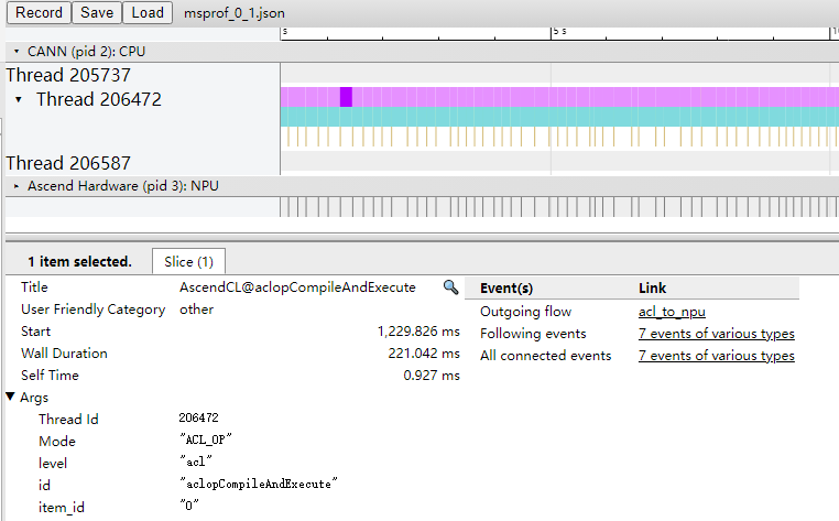
   • To open a timeline .json file, enter chrome://tracing in the address box of Google Chrome, drag the file to the blank space to open it, and press the shortcut keys (w: zoom in; s: zoom out; a: move left; d: move right) on the keyboard to view it. You can view the timeline information of the current AI task in a .json file, such as the API call timeline during task running, as shown in Figure 1.
     Figure 1 Viewing a .json file
     
   • You can directly open a summary .csv file to view it. You can view the software and hardware data during AI task running in a .csv file, such as the time required by each operator to run on the AI processor software and hardware. You can quickly find the required information by sorting fields, as shown in Figure 2.
     Figure 2 Viewing a .csv file
     

Collecting, Parsing, and Exporting Profile Data ( Ascend RC )

1. Log in to the operating environment and go to the /var directory where msprof is installed.
2. Run the following command to collect profile data:

   ./msprof --output=<path> <app>

   Example command:

   ./msprof --output=/home/projects/output /home/projects/MyApp/out/main

   Table 3 Command-line options

   Option	Description	Optional/Required
   --output=<path>	Directory for storing the collected profile data. The value defaults to the current directory.	Optional
   <app>	Add the AI task execution command to the end of the msprof command as required to pass the user application or execution script.	Required

   After the command is executed, the PROF_XXX directory is generated in the directory specified by --output. The directory structure is as follows:

   1 2 3 4 5 6

   ├── device_{id} │ ├── data │ └── ... └── host │ ├── data │ └── ...

3. Upload the PROF_XXX directory to the development environment where the tool is installed, and run the following command to parse data:

   msprof --export=on --output=<dir>

   Option	Description	Optional/Required
   --export	Profile data parsing and export. The value can be on or off (default). To export data of a specific model (model ID) or iteration (iteration ID), run the msprof --export command again to configure the --model-id and --iteration-id options after the msprof profiling command is executed. The PROF_XXX files that are not parsed are automatically parsed and then exported. Example: msprof --export=on --output=/home/HwHiAiUser	Required
   --output	Directory for storing the profile data file. The value must be PROF_XXX or the parent directory of PROF_XXX, for example, /home/HwHiAiUser/profiler_data/PROF_XXX.	Required

   Data files are added to the PROF_XXX directory. The directory structure is as follows:

   1 2 3 4 5 6 7 8 9

   ├── device_{id} │ ├── data ├── host │ ├── data │ └── ... └── mindstudio_profiler_output ├── xx_*.csv ├── xx_*.json ...

4. Access the mindstudio_profiler_output directory to view corresponding profile data files.

   For details about the files collected by default, see Table 4.

   Table 4 Profile data files collected by msprof by default

   File Name	Description
   msprof_*.json	Timeline report.
   step_trace_*.json	Iteration trace data, which records the time required for each iteration. This profile data file does not exist in single-operator scenarios.
   op_summary_*.csv	AI Core and AI CPU operator data.
   op_statistic_*.csv	Number of times that the AI Core and AI CPU operators are called and the time consumption.
   step_trace_*.csv	Iteration trace data. This profile data file does not exist in single-operator scenarios.
   task_time_*.csv	Task Scheduler data.
   fusion_op_*.csv	Operator fusion summary in a model. This profile data file does not exist in single-operator scenarios.
   api_statistic_*.csv	Time spent by API execution at the CANN layer.
   Note: The asterisk (*) indicates the timestamp.

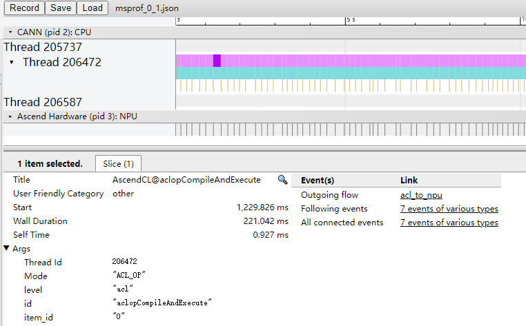
   • To open a timeline .json file, enter chrome://tracing in the address box of Google Chrome, drag the file to the blank space to open it, and press the shortcut keys (w: zoom in; s: zoom out; a: move left; d: move right) on the keyboard to view it. You can view the timeline information of the current AI task in a .json file, such as the API call timeline during task running, as shown in Figure 3.
     Figure 3 Viewing a .json file
     
   • You can directly open a summary .csv file to view it. You can view the software and hardware data during AI task running in a .csv file, such as the time required by each operator to run on the AI processor software and hardware. You can quickly find the required information by sorting fields, as shown in Figure 4.
     Figure 4 Viewing a .csv file
     

Performance Analysis

The preceding information shows that there are many profile data files and the analysis methods are flexible. The following introduces several important files and corresponding analysis methods.

• View the msprof*.json file to check the timeline information of an AI task from a holistic perspective and analyze possible bottlenecks.
  Figure 5 Example of the msprof*.json file
  

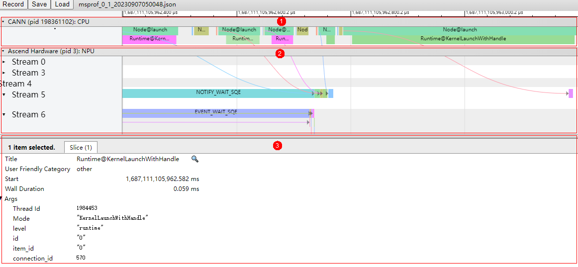
  • Area 1: data at the CANN layer, including the time consumption data of components (such as Runtime) and nodes (operators).
  • Area 2: bottom-layer NPU data, including the time consumption data and iteration trace data of each task stream under Ascend Hardware and other AI processor system data.
  • Area 3: details about each operator and API in a timeline (displayed when you click a timeline color block).

  From the above figure, we can roughly analyze the APIs, operators, and task streams that take a long time. Then, find the corresponding delivery relationship based on the arrow directions, analyze the specific bottom-layer tasks that take a lot of time during the inference process, check the time-consuming APIs and operators in area 3, and perform quantitative analysis based on the .csv file to locate the performance bottlenecks.

• Analyze the op_statistic_*.csv file to obtain the total calling time and total number of calls of each type of operators, check whether there are any operators with long total execution time, and analyze whether there is any optimization space for these operators.
  Figure 6 Example of the op_statistic_*.csv file
  

  You can sort the operators by Total Time to find out which type of operators takes a long time.

• Analyze the op_summary_*.csv file to obtain the basic information and time consumption of a specific operator, find the operator with high time consumption, and check whether there is any optimization space for the operator.
  Figure 7 Example of the op_summary_*.csv file
  

  The Task Duration field specifies the operator time consumption. You can sort operators by Task Duration to find time-consuming operators, or sort them by Task Type to view the time-consuming operators running on different cores (AI Core and AI CPU).