


基于香橙派AIpro+MindSpore实现情感分类任务
发表于: 2025/04/24
基于香橙派AIpro+MindSpore实现情感分类任务
01引言
情感分类是自然语言处理中的经典任务,是典型的分类问题。本案例使用MindSpore实现一个基于RNN网络的情感分类模型,实现如下的效果:
输入: This film is terrible
正确标签: Negative
预测标签: Negative
输入: This film is great
正确标签: Positive
预测标签: Positive
02环境准备
开发者拿到香橙派开发板后,首先需要进行硬件资源确认,镜像烧录及CANN和MindSpore版本的升级,才可运行该案例,具体如下:
硬件: 香橙派AIpro 16G 8-12T开发板
镜像: 香橙派官网ubuntu镜像
CANN:8.0.RC3.alpha002
MindSpore: 2.4.10
1、镜像烧录
运行该案例需要烧录香橙派官网ubuntu镜像,烧录流程参考昇思MindSpore官网--香橙派开发专区--环境搭建指南--镜像烧录章节,注意官网链接示例镜像与本案例镜像有所区别,以本案例要求为准,注意区分
2、CANN升级
CANN升级参考昇思MindSpore官网--香橙派开发专区--环境搭建指南--CANN升级章节。本案例的CANN版本要求是8.0RC3alpha002,注意官网链接示例升级版本与本案例所需版本有所区别,以本案例要求为准,注意区分。
3、MindSpore升级
MindSpore升级参考昇思MindSpore官网--香橙派开发专区--环境搭建指南--MindSpore升级章节,本案例的mindspore版本要求是2.4.10,注意官网链接示例升级版本与本案例所需版本有所区别,以本案例要求为准,注意区分。
03实验过程
1.设置运行环境
import mindspore mindspore.set_context(max_device_memory="2GB", mode=mindspore.GRAPH_MODE, device_target="Ascend", \jit_config={"jit_level":"O2"}, ascend_config={"precision_mode":"allow_mix_precision"})
2.数据处理
1、数据下载模块
为了方便预训练词向量的下载,首先设计数据下载模块,实现可视化下载流程,并保存至指定路径。数据下载模块使用requests库进行http请求,并通过tqdm库对下载百分比进行可视化。此外针对下载安全性,使用IO的方式下载临时文件,而后保存至指定的路径并返回。
(1)tqdm、requests安装
!pip install tqdm requests(2)定义下载函数
import os
import shutil
import requests
import tempfile
from tqdm import tqdm
from typing import IO
# from pathlib import Path

# 指定保存路径
cache_dir = os.getcwd() + '/mindspore_examples'

def http_get(url: str, temp_file: IO):
    """使用requests库下载数据,并使用tqdm库进行流程可视化"""
    req = requests.get(url, stream=True)
    content_length = req.headers.get('Content-Length')
    total = int(content_length) if content_length is not None else None
    progress = tqdm(unit='B', total=total)
    for chunk in req.iter_content(chunk_size=1024):
        if chunk:
            progress.update(len(chunk))
            temp_file.write(chunk)
    progress.close()

def downloads(file_name: str, url: str):
    """下载数据并存为指定名称"""
    if not os.path.exists(cache_dir):
         os.makedirs(cache_dir)
    cache_path = os.path.join(cache_dir, file_name)
    cache_exist = os.path.exists(cache_path)
    if not cache_exist:
          with tempfile.NamedTemporaryFile() as temp_file:
              http_get(url, temp_file)
              temp_file.flush()
              temp_file.seek(0)
              with open(cache_path, 'wb') as cache_file:
                  shutil.copyfileobj(temp_file, cache_file)
return cache_path2、加载预训练词向量
预训练词向量是对输入单词的数值化表示,通过nn.Embedding层,采用查表的方式,输入单词对应词表中的index,获得对应的表达向量。 因此进行模型构造前,需要将Embedding层所需的词向量和词表进行构造。这里我们使用Glove(Global Vectors for Word Representation)这种经典的预训练词向量, 其数据格式如下:
| Word | Vector |
|---|---|
| the | 0.418 0.24968 -0.41242 0.1217 0.34527 -0.044457 -0.49688 -0.17862 -0.00066023 ... |
| , | 0.013441 0.23682 -0.16899 0.40951 0.63812 0.47709 -0.42852 -0.55641 -0.364 ... |
我们直接使用第一列的单词作为词表,使用dataset.text.Vocab将其按顺序加载;同时读取每一行的Vector并转为numpy.array,用于nn.Embedding加载权重使用。具体实现如下:
import zipfile
import numpy as np
import mindspore.dataset as ds

def load_glove(glove_path):
    glove_100d_path = os.path.join(cache_dir, 'glove.6B.100d.txt')
    if not os.path.exists(glove_100d_path):
        glove_zip = zipfile.ZipFile(glove_path)
        glove_zip.extractall(cache_dir)

    embeddings = []
    tokens = []
    with open(glove_100d_path, encoding='utf-8') as gf:
        for glove in gf:
              word, embedding = glove.split(maxsplit=1)
              tokens.append(word)
              embeddings.append(np.fromstring(embedding, dtype=np.float32, sep=' '))
    # 添加 <unk>, <pad> 两个特殊占位符对应的embedding
    embeddings.append(np.random.rand(100))
    embeddings.append(np.zeros((100,), np.float32))

    vocab = ds.text.Vocab.from_list(tokens, special_tokens=["<unk>", "<pad>"], special_first=False)
    embeddings = np.array(embeddings).astype(np.float32)
return vocab, embeddings由于数据集中可能存在词表没有覆盖的单词,因此需要加入<unk>标记符;同时由于输入长度的不一致,在打包为一个batch时需要将短的文本进行填充,因此需要加入<pad>标记符。完成后的词表长度为原词表长度+2。
下载Glove词向量,并加载生成词表和词向量权重矩阵
glove_path = downloads('glove.6B.zip', 'https://mindspore-website.obs.myhuaweicloud.com/notebook/datasets/glove.6B.zip')
vocab, embeddings = load_glove(glove_path)
len(vocab.vocab())使用词表将the转换为index id,并查询词向量矩阵对应的词向量
idx = vocab.tokens_to_ids('the')
embedding = embeddings[idx]
idx, embedding3、模型构建
用于情感分类的模型结构,首先需要将输入文本(即序列化后的index id列表)通过查表转为向量化表示,此时需要使用nn.Embedding层加载Glove词向量;然后使用RNN循环神经网络做特征提取;最后将RNN连接至一个全连接层,即nn.Dense,将特征转化为与分类数量相同的size,用于后续进行模型优化训练。整体模型结构如下:
nn.Embedding -> nn.RNN -> nn.Dense
这里我们使用能够一定程度规避RNN梯度消失问题的变种LSTM(Long short-term memory)做特征提取层。下面对模型进行详解:
1.Embedding
Embedding层又可称为EmbeddingLookup层,其作用是使用index id对权重矩阵对应id的向量进行查找,当输入为一个由index id组成的序列时,则查找并返回一个相同长度的矩阵,例如:
embedding = nn.Embedding(1000, 100) # 词表大小(index的取值范围)为1000,表示向量的size为100
input shape: (1, 16) # 序列长度为16
output shape: (1, 16, 100)
这里我们使用前文处理好的Glove词向量矩阵,设置nn.Embedding的embedding_table为预训练词向量矩阵。对应的vocab_size为词表大小400002,embedding_size为选用的glove.6B.100d向量大小,即100。
2、RNN(循环神经网络)
循环神经网络(Recurrent Neural Network, RNN)是一类以序列(sequence)数据为输入,在序列的演进方向进行递归(recursion)且所有节点(循环单元)按链式连接的神经网络。下图为RNN的一般结构:
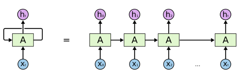
上图左侧为一个RNN Cell循环,右侧为RNN的链式连接平铺。实际上不管是单个RNN Cell还是一个RNN网络,都只有一个Cell的参数,在不断进行循环计算中更新。
由于RNN的循环特性,和自然语言文本的序列特性(句子是由单词组成的序列)十分匹配,因此被大量应用于自然语言处理研究中。下图为RNN的结构拆解:
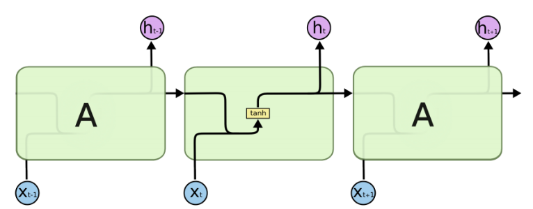
NN单个Cell的结构简单,因此也造成了梯度消失(Gradient Vanishing)问题,具体表现为RNN网络在序列较长时,在序列尾部已经基本丢失了序列首部的信息。为了克服这一问题,LSTM(Long short-term memory)被提出,通过门控机制(Gating Mechanism)来控制信息流在每个循环步中的留存和丢弃。下图为LSTM的结构拆解:
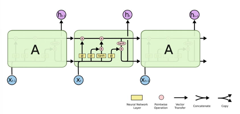
本案例我们选择LSTM变种而不是经典的RNN做特征提取,来规避梯度消失问题,并获得更好的模型效果。下面来看MindSpore中nn.LSTM对应的公式:

这里nn.LSTM隐藏了整个循环神经网络在序列时间步(Time step)上的循环,送入输入序列、初始状态,即可获得每个时间步的隐状态(hidden state)拼接而成的矩阵,以及最后一个时间步对应的隐状态。我们使用最后的一个时间步的隐状态作为输入句子的编码特征,送入下一层。
3、Dense
在经过LSTM编码获取句子特征后,将其送入一个全连接层,即nn.Dense,将特征维度变换为二分类所需的维度1,经过Dense层后的输出即为模型预测结果。
import math
import mindspore as ms
import mindspore.nn as nn
import mindspore.ops as ops
from mindspore.common.initializer import Uniform, HeUniform

class RNN(nn.Cell):
    def __init__(self, embeddings, hidden_dim, output_dim, n_layers,
                   bidirectional, pad_idx):
        super().__init__()
        vocab_size, embedding_dim = embeddings.shape
        self.embedding = nn.Embedding(vocab_size, embedding_dim, embedding_table=ms.Tensor(embeddings), padding_idx=pad_idx)
        self.rnn = nn.LSTM(embedding_dim,
                             hidden_dim,
                             num_layers=n_layers,
                             bidirectional=bidirectional,
                             batch_first=True)
        weight_init = HeUniform(math.sqrt(5))
        bias_init = Uniform(1 / math.sqrt(hidden_dim * 2))
        self.fc = nn.Dense(hidden_dim * 2, output_dim, weight_init=weight_init, bias_init=bias_init)

    def construct(self, inputs):
      embedded = self.embedding(inputs)
      _, (hidden, _) = self.rnn(embedded)
      hidden = ops.concat((hidden[-2, :, :], hidden[-1, :, :]), axis=1)
      output = self.fc(hidden)
      return output
模型实例化
hidden_size = 256
output_size = 1
num_layers = 2
bidirectional = True
pad_idx = vocab.tokens_to_ids('<pad>')

model = RNN(embeddings, hidden_size, output_size, num_layers, bidirectional, pad_idx)
4、模型加载
使用MindSpore提供的Checkpoint加载和网络权重加载接口:1.将保存的模型Checkpoint加载到内存中,2.将Checkpoint加载至模型。
# download ckpt
from download import download
rnn_url = "https://modelers.cn/coderepo/web/v1/file/MindSpore-Lab/cluoud_obs/main/media/examples/mindspore-courses/orange-pi-online-infer/07-RNN/sentiment-analysis.ckpt"
path = "./sentiment-analysis.ckpt"
ckpt_path = download(rnn_url, path, replace=True)

param_dict = ms.load_checkpoint(ckpt_path)
ms.load_param_into_net(model, param_dict)load_param_into_net接口会返回模型中没有和Checkpoint匹配的权重名,正确匹配时返回空列表。
5、自定义输入测试
最后我们设计一个预测函数,实现开头描述的效果,输入一句评价,获得评价的情感分类。具体包含以下步骤:
- 将输入句子进行分词;
- 使用词表获取对应的index id序列;
- index id序列转为Tensor;
- 送入模型获得预测结果;
- 打印输出预测结果。
具体实现如下:
score_map = {
      1: "Positive",
      0: "Negative"
     }

def predict_sentiment(model, vocab, sentence):
    model.set_train(False)
    tokenized = sentence.lower().split()
    indexed = vocab.tokens_to_ids(tokenized)
    tensor = ms.Tensor(indexed, ms.int32)
    tensor = tensor.expand_dims(0)
    prediction = model(tensor)
    return score_map[int(np.round(ops.sigmoid(prediction).asnumpy()))]
最后我们预测开头的样例,可以看到模型可以很好地将评价语句的情感进行分类。
predict_sentiment(model, vocab, "This film is terrible")predict_sentiment(model, vocab, "This film is great")04实验视频
05实验总结
本实验在香橙派AIpro开发板上实现情感分类分类任务,通过本课程的学习,您可以了解情感分类任务的基本概念,掌握RNN基本结构、MindSpore搭建RNN网络、能够自己动手在香橙派AIpro开发板上进行案例发复现。